Last time we talked about figuring out what we want machine learning to do to be more important than how to do it. So before we jump into how to build a machine learning pipeline in the SnapLogic Elastic Integration Platform, let’s talk about what we are doing.
One application that is useful across a variety of industries and use-cases is anomaly detection. As the name implies, anomaly detection is designed to find data that is anomalous, or abnormal. This could be used to find evidence of malicious hacking, to identify failing software, implement quality control, clean data coming from IoT sensors, etc. Whatever the motivation, the first step is training the system. (The zeroth step is identifying the proper data source to use.) When you are satisfied with the detector’s performance (by testing it on data it hasn’t “seen”), you deploy the system to inspect data – likely streaming data.
Anomaly detection systems have long been implemented without machine learning, generally by having rules of thumb. Widgets outside of a certain tolerance are rejected; a server whose CPU is at 95% utilization for more than a minute is examined for a possible run-away process; a thermostat reporting temperatures outside of 0 to 120 degrees Fahrenheit is checked for a malfunction. Machine learning adds the ability to create these rules automatically, with more clearly defined trade-offs, and with the possibility of periodically retraining the model if we have reason to believe the process will change over time.
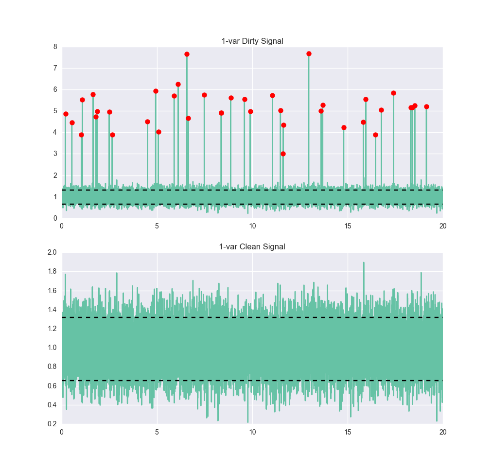
Let’s take a look at a very simple signal. Below we see a signal that has some noise, but it’s pretty clear that it should be about 1, with a six-sigma range of roughly between 0.4 and 1.6. Now we train an anomaly detector on it, using a single-class support vector machine (SVM). The details of how an SVM works are beyond the scope of this post, but if you’re interested, O’Reilly Media has an excellent interactive post by Jake VanderPlas on the subject, as does the scikit-learn documentation. For our purposes, the SVM is trained by giving it normal data. We don’t have to get it examples of anomalous data. Having trained it, let’s get it some dirtier data and see how it performs:

true_pos:       17964

true_neg:       39

false_pos:      1997

false_neg:      0

accuracy:       0.90015

precision:      0.89995

recall:         1.0

F1:             0.94734
The anomaly/not-anomaly boundaries have been plotted on this graph as the black horizontal lines. For an off-the-shelf algorithm with little tuning, this isn’t bad. We catch all of the anomalies, which is good, but we’re also classifying about 10% of the normal points as anomalies. If we had used two classes (i.e., by training on the set with anomalies, provided we could identify them) we would probably get much better performance – in particular, many fewer false-positives.
Anomaly detectors really start to shine when the anomaly is not just one variable behaving badly. For example, imagine monitoring the incoming connections to a web server and its CPU usage. We generally expect these to be linearly related. If CPU usage is high when connections are low, we’d be concerned about a process gone bad or a possible security breach. If connections are high but CPU usage is low, maybe it’s because our main application crashed and users and just being served error pages. Either way, knowing either CPU usage or incoming connections is enough to characterize an anomaly; we need to examine both, as illustrated below*:

Train Data, (clean):            Test Data Set:

true_pos:       18999           true_pos:       4668

true_neg:       0               true_neg:       64

false_pos:      0               false_pos:      23

false_neg:      1001            false_neg:      245

accuracy:       0.94995         accuracy:       0.9464

precision:      1.0             precision:      0.99509

recall:         0.94995         recall:         0.95013

F1:             0.97433         F1:             0.97209
In the next two installments of this series, we’re first going to build out the pipeline for anomaly detection based on the simple one-variable anomaly detector. For the first part, we’re going to assume we have an anomaly detection Snap, but not go into any details about it. In the last part, we’re going to come back to this black-box Snap, and show how we can quickly setup an elastic-scaling anomaly detector on Azure ML that is exposed to us as a simple REST service. Finally, if you’re curious about the graphs created in this post, we’ve posted the Python code in a GitHub repository for you to look at. There are two scripts and one IPython / Jupyter notebook. Both are in rough form (pull requests welcome!) but are a good starting point for further exploration.
* You could also note that you care about the ratio between the two variables – call them x1 and x2 – and so you could create a single variable SVM on x3 by letting x3 = x1 / x2. That is true, but note that (a) you’ve just manually interjected some knowledge of the process into the system (the linear relationship) and (b) as x2 goes to 0, x3 goes to infinity, which is always problematic.


